The Lumenaut Monte Carlo Risk Simulation package provides a range of tools that enable the user to easily and quickly build interactive monte carlo risk simulation models natively in Excel.
If you have an existing Excel model or building one from scratch, it is simple to place a Monte Carlo Simulation on top of this. There are no special formulas required, just point and click on the individual cells you wish to mark in the analysis and set the parameters.
Monte Carlo Analysis is increasingly being used in all fields and industries where a better appreciation of the actual likelihood of obtaining certain results such as profitability (Business Analysis, Project Risk Assessment), Tolerances (Manufacturing and Six Sigma), failures (engineering), for example, is required.
Example of a simple financial model
The basic Model, Bob wishes to examine the likely profitability of his new product idea. So he first builds his financial predictive model in Excel. However, all he gets out of this model is a single answer what he needs is an ideal of the possible range of profits he can make and their probabilities.
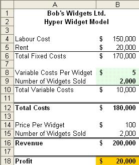
Bob decides to use Monte Carlo analysis as this will enable him to ascribe probability distributions to his input variables
Using the Risk Input Form, below, he chooses suitable probability distribution for his input parameters. These cells are marked in green by Lumenaut.
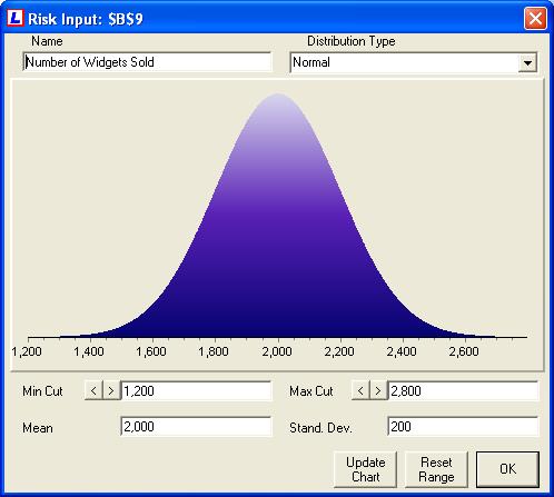
The following statistical distributions are available:
- Beta
- Binomial
- Exponential
- Extreme Value
- Gamma
- Geometric
- Lognormal
- Logistic
- Negative Binomial
- Normal
- Poisson
- Triangular
- Uniform
- Weibul
Using the Output Form, opposite, he selects the output cells in the model, in this case profitability, shown in orange above by Lumenaut.
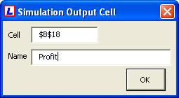
It is possible to give each individual output cell an easy to identify name.
Finally the model can be run via the Run Simulation Form, it is possible to set the number of iterations for the simulation from 1,000 to millions.
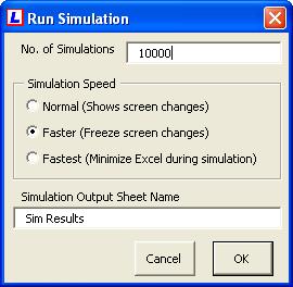
The speed of the simulation can be adjust while individual names can be given to the result sheet.
The results of the simulation are printed in a result sheet.
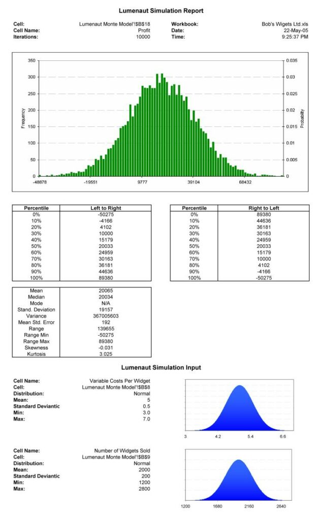
The probability distribution for the output variables are given in green below which are found the frequency distribution tables.
Univariate statistics reported include Mean, Median, Mode, Standard Deviation, Variance, Mean Standard Error, Variance, Range, Max , Min , Skewness and Kurtosis.
The input distributions are shown in blue.
For another example Oil and Gas Reserve Estimation example using Lumenaut can be downloaded here pdf and Excel